Persistent Orthogonality of Trained Weight Matrices
TL;DR
-
Implicit Regularization: Gradient descent isn’t just a blind search; it respects the initial parameterization.
The algorithm gently changes the weights without violently breaking the beneficial structure we started with. -
Training Stability: Orthogonal matrices preserve norms, which helps prevent exploding or vanishing gradients.
The derivation shows that training maintains this property, explaining why orthogonal initialization often leads to more stable training. -
A New Perspective: It suggests that carefully chosen initializations aren’t just a good starting point, they can define a subspace or a manifold within which the entire optimization process occurs.
I was surprised to notice that weight matrices initialized orthogonally tend to remain nearly orthogonal even after training. This got me into thinking, even after applying nonlinear activations and running gradient descent over and over, that structure should have collapsed.
Experimenting with generated data and few steps of training was somehow preserving the orthogonality but this wasn't a reasonable explanation. I was looking for some good mathematical proof of this persistence.
Then I recalled Gilbert Strang's discussion on Matrix Perturbation Theory "how small changes in a matrix affect its properties.". That instantly clicked the thought, perhaps training won’t destroy or change the matrix completely but only perturbs it in a way that the structure remains intact. And the only way to track these changes is to measure how much drifts away from identity matrix (as weights matrices are initialized orthogonally, before training equals identity matrix)
Playing around with gradient descent
If I apply this repeatedly i'll get something like this
So basically after this unrolling of gradients I can write gradient equation in terms of weight matrix before training and after training as follows
If I use gradient clipping technique, which will basically set a threshold for gradient values like this:
then by triangle inequality and submultiplicativity properties I can write the gradient descent equation as
Measuring how far has the weight matrix gone from identity
To find out how far the weight matrix is from being and identity, I have to calculate the value of
For this I used a very common matrix identity in matrix perturbation theory
it can be easily verified that LHS and RHS of this equation are same (which is left as an exercise for reader)
Now by applying norms and making use of submultiplicativity property and triangle inequality, the following equation can be derived
And since
I can re-write entire equation as
Using this matrix identity for weights
Let (A = W(t)), (B = W(0)). Then
I already know that
Substituting this in above equation
The norm of matrix W(0) will be equal to 1, so the equation will be
Thus an upper bound for how much the weight matrix will differ from orthogonally initialized matrix after training is obtained
I started with a simple observation: orthogonality persists.
Through matrix perturbation theory, I found a mathematical bound for this phenomenon:
At first glance, this bound seems circular, it requires knowing , a property of the trained matrix I was trying to understand.
But this is where the initial observation and the theory converge beautifully.
The very fact that we observe to be nearly orthogonal means its singular values are all near , so .
This collapses the bound into a much more intuitive form:
Fascinating Implications
-
Implicit Regularization: Gradient descent isn’t just a blind search; it respects the initial parameterization.
The algorithm gently changes the weights without violently breaking the beneficial structure we started with. -
Training Stability: Orthogonal matrices preserve norms, which helps prevent exploding or vanishing gradients.
The derivation shows that training maintains this property, explaining why orthogonal initialization often leads to more stable training. -
A New Perspective: It suggests that carefully chosen initializations aren’t just a good starting point, they can define a subspace or a manifold within which the entire optimization process occurs.
Practically testing things
A mathematical bound is only as interesting as its connection to reality.
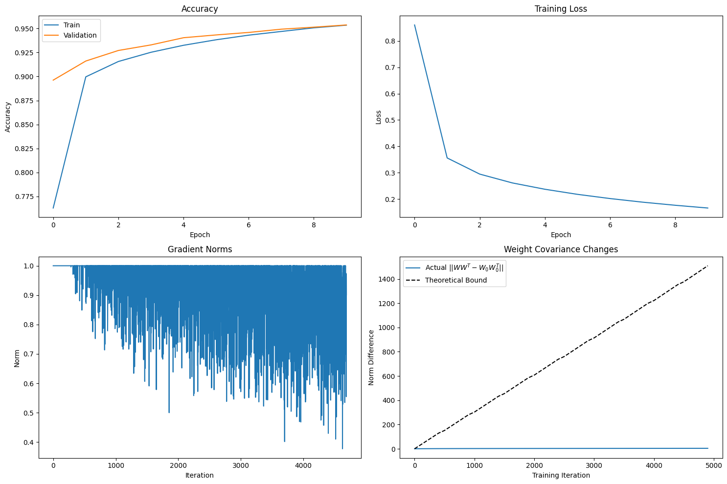
To test the derivation, I trained a simple classifier on MNIST using orthogonally initialized weights and gradient clipping ().
The theory gives a strict upper limit:
After training for 10 epochs, the model reached a respectable 95.4% validation accuracy.
Let's look at the final numbers:
| Metric | Value |
|---|---|
| Validation Accuracy | 0.9537 |
| Final Gradient Norm | 0.9009 |
| Final Weight Norm | 16.3235 |
| Actual Deviation | 4.1151 |
| Theoretical Upper Bound | 1508.95 |
| Bound / Actual Ratio | 366.68 |
What does this mean?
-
The Bound Holds: The most important result is that the actual deviation () is indeed less than the calculated upper bound ().
-
The Bound is Conservative: As is common in theoretical analysis, the bound is not tight.
It's a worst-case scenario that assumes all gradient updates conspire in the most destructive direction.
In practice, updates are noisy and often cancel each other out, leading to a much smaller actual change. -
The Real Story is in the Trend:
The bound's linear growth with and its dependence on are the key insights.
The fact that the actual deviation remains orders of magnitude smaller shows that training is a remarkably stable perturbation process, not a destructive one.
Hope you got some good insights :)
Have a great day!